Basic OSS Architecture
The purpose of this project is to showcase the power of open source tools when designing a data and analytics system. I will be walking through my workflow step by step, and including both images, code, and notes.
Project Initialization
First Steps
Let’s start from scratch, a blank VS Code IDE. I’ll do everything from the command line, so make sure to open that up (Ctrl-`).
![]()
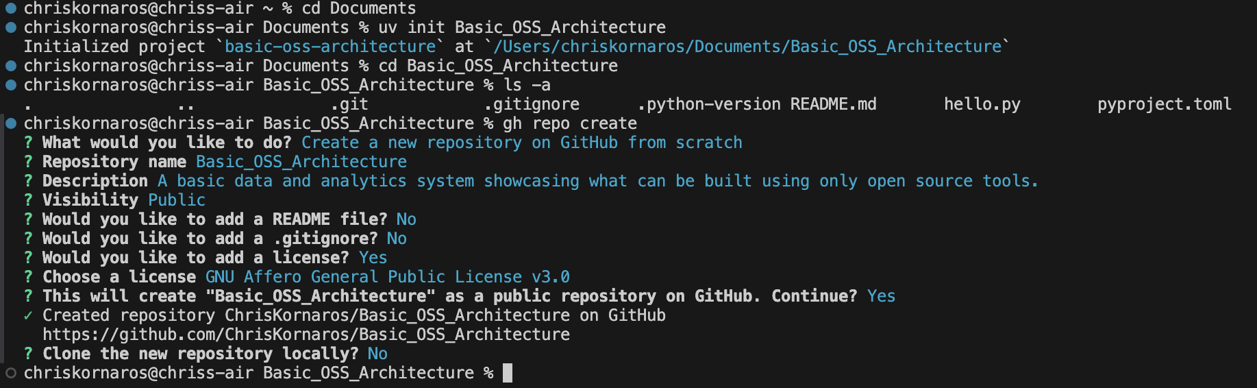
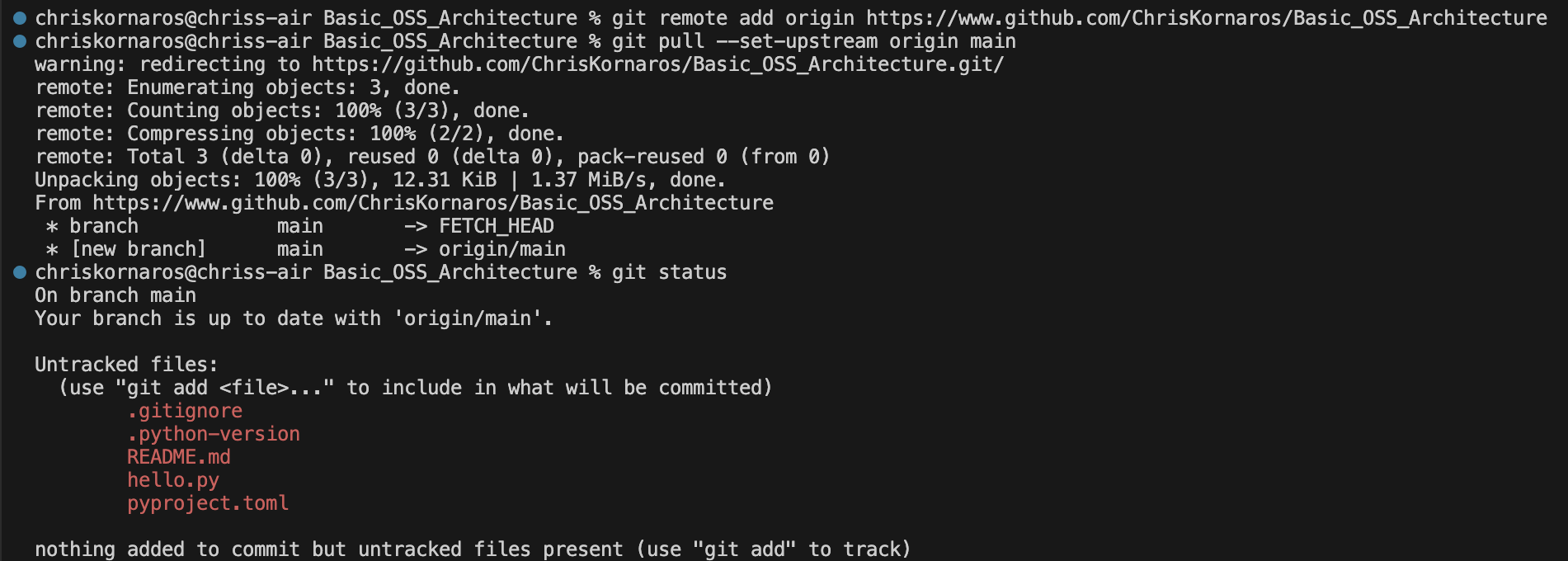
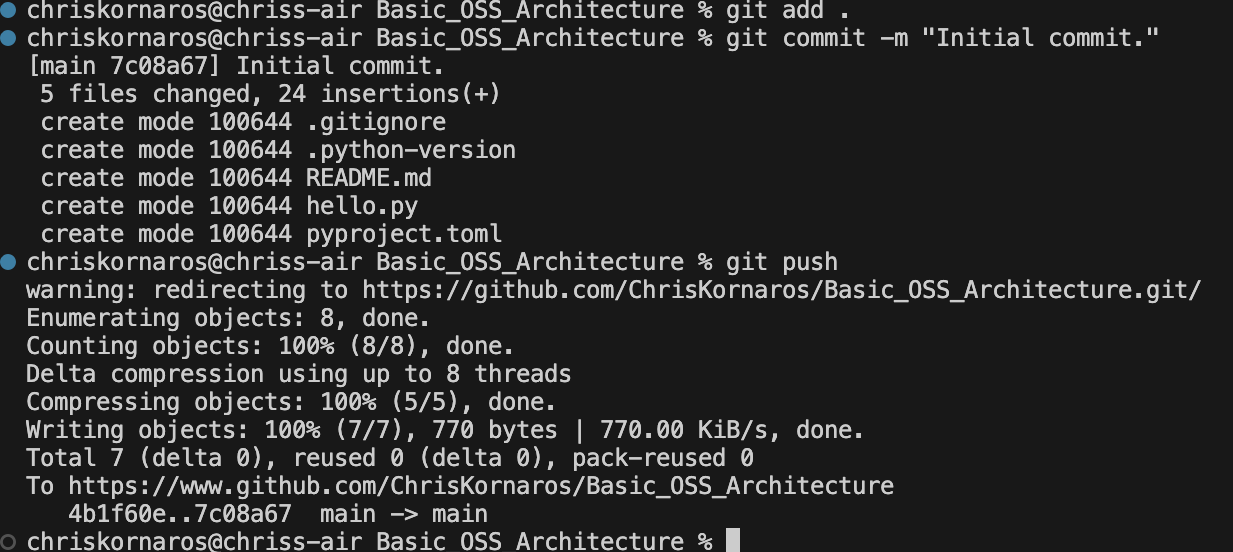
First, I begin in my home directory. Then, I change to my Documents directory, which I use for all of my projects. This is where I’ll begin creating the project directory and initializing the subsequent tools. As you’ll see below, I first initialize the uv repository and change into it. Then, I create the repo on GitHub (because I like generating the license then), pull (my global is set to merge), commit, and make the initial push. Then, I will initialize the Quarto project, to begin documentation as I work.
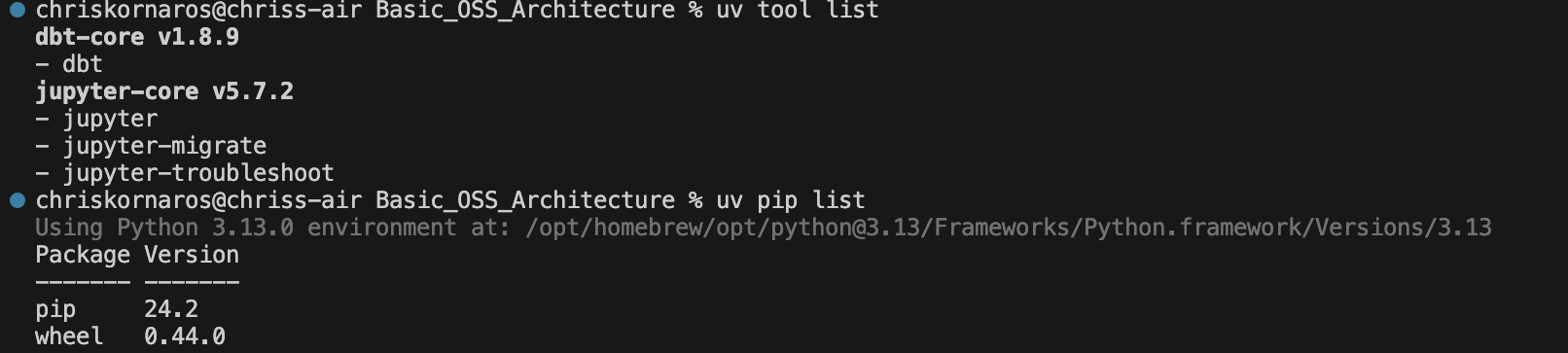 You can see here that I have both
 jupyter and dbt already installed. That’s because uv installs tools system wide, because these are typically used from the CLI. That being said, some CLI tools (like Quarto and DuckDB) in my experience don’t work with uv because it doesn’t install their executables.
Adding Quarto
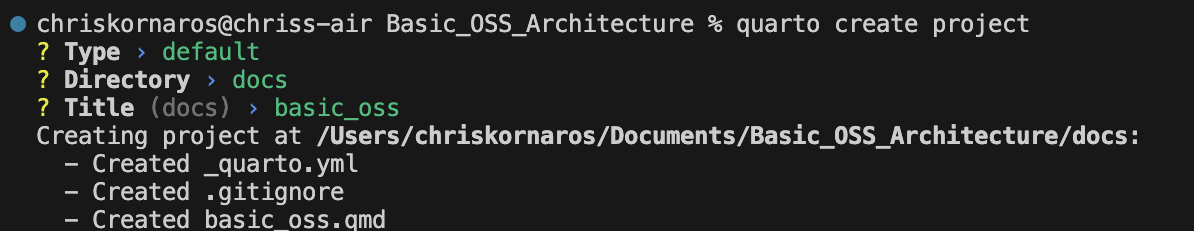
Now, it’s time to setup some extra functionality in the project. I’m going to be using Quarto for documentation, so I’ll run quarto create project. To learn more about Quarto and configuring your documentation in projects, checkout my guide. It’s a fantastic tool for building beautiful, robust documentation, even in enterprise production environments. Consider it for future papers, websites, dashboards, and reports.
That being said, if you are ever taking screenshots of your work and want to quickly move them into your images folder, you can do so from the CLI.

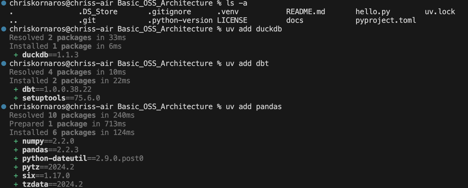
Now that you’ve done that, it’s time to start adding dependencies. As a heads up, don’t be surprised if you don’t see the uv.lock or the .venv objects in your directory right away, because uv doesn’t create those until you add dependencies. Simply run uv add to start adding them. Afterwards, the necessary requirements and lock files will update automatically. If you want to learn more, checkout my uv guide.
The Pyproject.toml file
Once that’s done, uv will update the general dependencies in the pyproject.toml file and the specific versions in uv.lock (think requirements.txt on steroids). The nice thing here, it only lists the actual package you needed, not everything else that the package requires. So, when you want to remove packages you can simply use uv remove and the individual package names listed here to remove everything in your environment. There’s an example below.
[project]
name = "basic-oss-architecture"
version = "0.1.0"
description = "Add your description here"
readme = "README.md"
requires-python = ">=3.13"
dependencies = [
    "dbt-core>=1.9.1",
    "dbt-duckdb>=1.9.1",
    "dbt-postgres>=1.9.0",
    "duckdb>=1.1.3",
    "fsspec>=2024.10.0",
    "great-expectations>=0.18.22",
    "jupyter>=1.1.1",
    "pandas>=2.2.3",
    "pytest>=8.3.4",
    "quarto>=0.1.0",
    "requests>=2.32.3",
    "ruff>=0.8.4",
]
Using .gitignore effectively
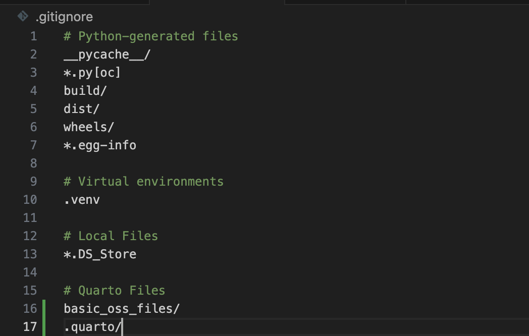
You probably noticed, but when you initialize a project with uv it automatically creates a .gitignore file and populates it with basic files and directories which don’t need to be checked into source control (like .venv). I take this a step further, and add some Quarto specific files and directories too, .quarto and _files folders. Managing this file effectively can drastically reduce the file size of your commits.
Below is an example of my file at this early project stage.
Initializing a Data Environment
Now, you’ll be setting up dbt. Similar to the other CLI tools, dbt uses the dbt init command to create the folder structure necessary for the program to be effective. As you can see below, the process is very easy. You’ll only enter a name for your project, which will (case sensitively) become the name of the dbt directory. Next, I’ll walk through the fundamental pieces of a dbt project in depth.
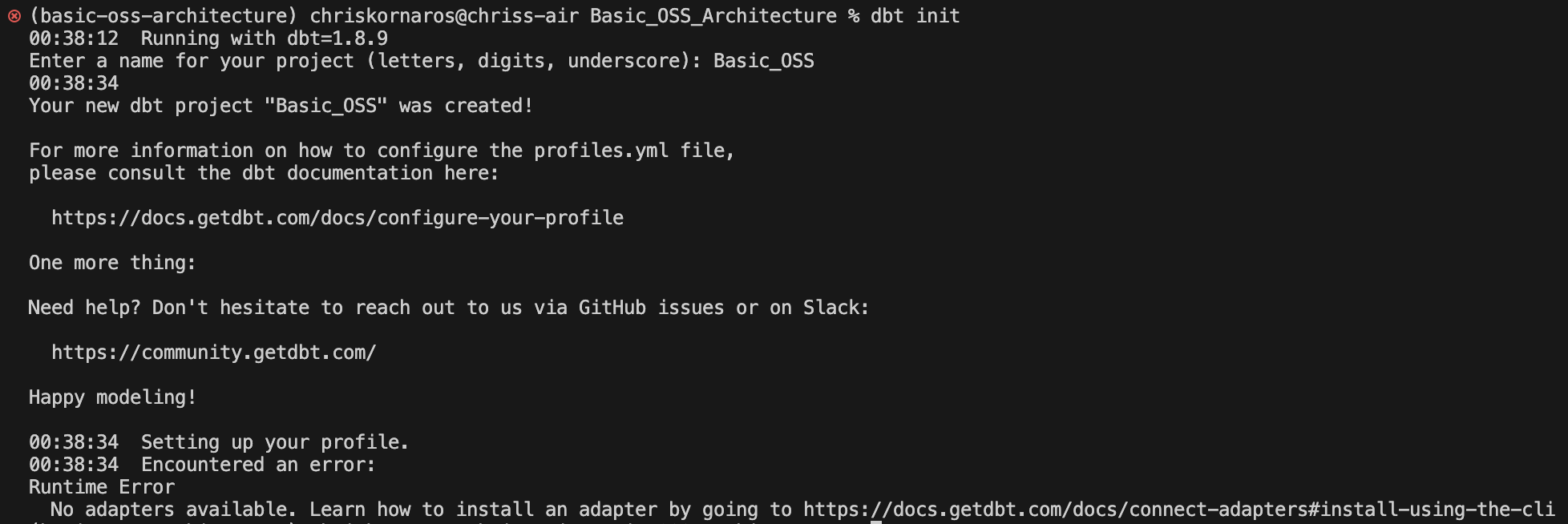
Due to some naming conventions and for simplicity, I later changed the name of the dbt projct in my environment to basic_oss. It’s easier to type when it’s all lowercase and it fits with the dbt naming conventions better. So, don’t be surprised if/when you see it later.
The Data Build Tool (dbt)
As I said, creating a dbt project is easy, but it can get confusing from here on out if you’re alone with the dbt documentation. In my experience, dbt initalizes a logs/ folder in the project root directory not the dbt root directory. So, I make sure to add that to the gitignore file, because I don’t think that needs to be checked into version control.
So, now that you’ve initialized your folder, let’s go through the basics:
Project Root: Basic_OSS
In the case of my project, the root folder is called Basic_OSS. Here, you’ll find the 6 subdirectories, a .gitignore file, a README.md file, and the dbt_project.yml file. The .gitignore can be deleted, because you have one in the project root directory, and for the same reason, so can the README. The dbt project file is the core of your entire data environment, in the same exact way that a _quarto.yml file is the core of your website, book, or documentation project.
This is where you’ll configure the actual structure and hierarchy of your environment, along with things like schemas or variables, or aliases.
Analyses
Contains the SQL files for any analysis done that are not part of the core models. Think of these as the SELECT statements for analytical queries, whereas models handle the DDL statements for database architects. Depending on your workflow, this folder could be unused.
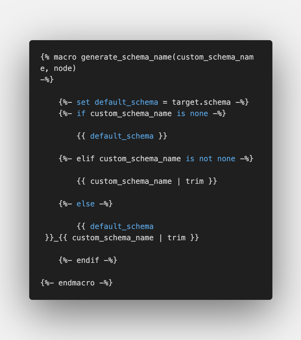
Macros
This is where you can store custom macros (functions) and reusable code written in either SQL or jinja. This is the Python package equivalent for SQL and it’s often used to ensure DRY (Don’t Repeat Yourself) principles for ETL and other database work.
By default, dbt will use main for the schema name. Furthermore, I found that even when specifying the schema in the YAML files, it would just append that to main either as main.example_schema.table or main_example_schema.table. For enterprise purposes, this behavior is intended and explained in dbt docs. For my purposes, I would rather the format and reference behavior be schema.table. To do this, I found and modified a custom macro.
Models
This is the core of dbt. Models are the SQL tables themselves, as well as the transformations when cleaning and aggregating data (from raw to reporting). If you have a raw schema (where the raw data is temporarily stored) and a clean schema (where cleaned data is persisted), you would have both a raw and clean folder within the models folder. Then, the individual queries would live within those subfolders as the actual tables and views.
It is where most of (if not all) your transformations live. So, can become computationally taxing if you aren’t careful.
Run with dbt run or dbt run --select {model_directory_name}.
Seeds
These are flat files containing static data used for mapping (or reference) data. Only use this if your project needs static data. For more on seeds.
Run with dbt seed.
Snapshots
Stores snapshot definitions for versioning and tracking changes in source data over time. These are commonly used for SCDs (slowly changing dimensions) or auditing.
Run with dbt snapshot.
Tests
Fairly self explanatory, but this folder contains custom, SQL-defined tests for your models. Dbt allows for both custom tests defined in .sql files and generic tests defined in a YAML. The tests run on various models are defined in the dbt_project.yml file.
Extra Notes
Dbt also has the docs/ and dbt_packages/ folders which are for advanced documentation and shareable, modularized code, respectively. Generally speaking, your workflow will really only involve the following parts of a dbt project:
models/tests/macros/dbt_project.yml
The others are optional and provide functionality, that while useful and powerful in many cases, is not always needed. Now that I’ve got the local directory all configured, it’s time to start building the container for my PostgreSQL instance (server, cluster, whatever you want to call it).
Docker and Containers
Docker is a powerful open-source platform that simplifies the process of developing, packaging, and deploying applications using containers, which are lightweight, portable environments. Unlike traditional virtualization, which replicates an entire computer system, containers virtualize at the operating system (OS) level, creating isolated spaces where applications run with all their dependencies. By isolating apps in containers, Docker ensures that each environment is consistent across different systems, reducing conflicts caused by mismatched dependencies. This approach accelerates development, enhances portability, and enables scalability, making Docker a cornerstone of modern microservices architectures and containerized workflows.
You can learn more about Docker either through their open source documentation or DataCamp’s course by Tim Sangster!
The Dockerfile and Configuring Your Image
The Dockerfile is the foundation of Docker image creation, serving as a script of instructions to define the environment and behavior of your containerized application. Each instruction in the Dockerfile builds on the previous one, forming layers that together create a Docker image.
A Dockerfile is composed of various instructions, such as:
FROM: Specifies the base image to start with. Always begin with this instruction.
FROM postgresRUN: Executes shell commands during the build process and creates a new layer.
RUN apt-get updateCOPY/ADD: Transfers files from your local system into the image.
COPY postgres-password.txt /usr/home/WORKDIR: Sets the working directory for subsequent instructions.
WORKDIR /usr/home/CMD: Specifies the default command to run when the container starts. Unlike
RUN,CMDis executed at runtime.CMD ["postgres"]
Optimizing Builds with Caching
Docker employs a layer-caching mechanism to optimize builds. Each instruction in the Dockerfile forms a layer, and Docker reuses unchanged layers in subsequent builds to save time. For example:
RUN apt-get update
RUN apt-get install -y libpq-dev
If you rebuild and these instructions remain unchanged, Docker uses cached results. However, if the base image or any instruction changes, the cache is invalidated for that layer and subsequent ones.
Reorder Dockerfile instructions to maximize cache efficiency. Place less frequently changing instructions higher in the file. Then, place the layers you need to test changes in more frequently, lower in the file.
Using Variables in Dockerfiles
Variables make Dockerfiles more flexible and maintainable.
ARG: Sets build-time variables.
ARG APP_PORT=5000 RUN echo "Application port: $APP_PORT"ARGvalues are accessible only during the build process.ENV: Sets environment variables for runtime.
ENV APP_ENV=productionThese variables persist after the image is built and can be overridden when running the container using the
--envflag.
Avoid storing sensitive data like credentials in ARG or ENV, as they are visible in the image’s history.
Security Best Practices
Use Official Images: Base your
Dockerfileon trusted, well-maintained images from sources like Docker Hub.Minimize Packages: Install only what your application needs to reduce potential vulnerabilities.
Avoid Root Users: Run applications with restricted permissions by creating a non-root user:
RUN useradd -m appuser
USER appuser
Update Regularly: Keep your base images and software dependencies up to date.
Write a PostgreSQL Dockerfile and Build the Image
Below is an example Dockerfile for setting up PostgreSQL, with specified user, password, and database name:
# Use an official PostgreSQL base image
FROM postgres

# Set environment variables from a local file
COPY .pg-password /etc/postgresql/.pg-password

# Read the password from the file and set it as an environment variable
RUN POSTGRES_PASSWORD=$(cat /etc/postgresql/.pg-password)

# Set additional environment variables
ENV POSTGRES_USER=chris
ENV POSTGRES_DB=test

# Expose the PostgreSQL port
EXPOSE 5432

# Run commands to configure the environment
RUN apt-get update && apt-get install -y \
    libpq-dev \
    && rm -rf /var/lib/apt/lists/*

# Start PostgreSQL service when the container runs
CMD ["postgres"]
For the purposes of simplicity in this guide, I’m just going to leave the POSTGRES_ variables as they are in the file. The password I’ll keep separate to demonstrate how that would work. That being said, after you’ve writen the image’s Dockerfile, you’ll build the image.
docker build -t test .If you need to remove the image at any point, first make sure there are no containers using it, then run the following:
docker rmi test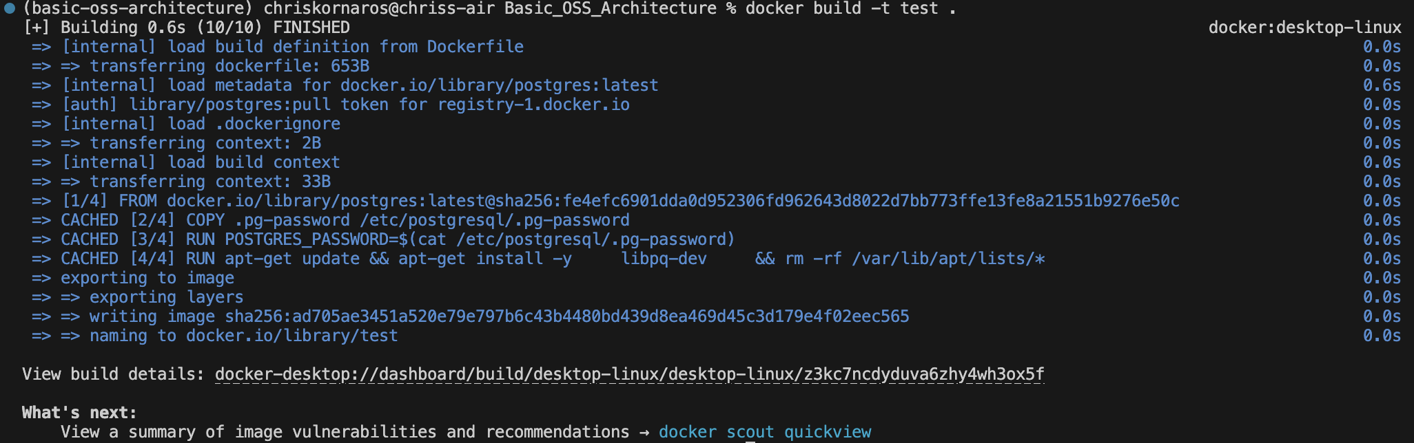
Running the Container
Next, to run the container, you’ll be adding a few flags, which I’ll explain below. For simplicity sake, it’s probably easiest to store this in a script somewhere and then execute that on start up. **Note** to myself: Add a section on writing local scripts/executables like this later on in the guide.
docker run \
  --name pg_test \
  -e POSTGRES_PASSWORD_FILE=/etc/postgresql/.pg-password \
  -e POSTGRES_USER=chris \
  -e POSTGRES_DB=test \
  -p 5432:5432 \
  test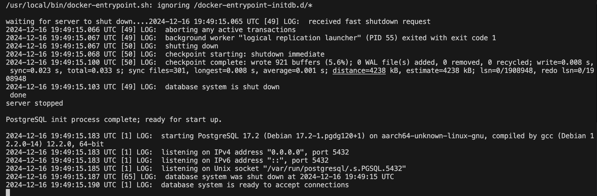
Flags Explained
The code above will run a container using the Docker image test as the base.
- The container will have the
--namepg_test - You’ll use the file located at
/etc/postgresql/.pg-passwordto define thePOSTGRES_PASSWORD_FILEenvironment variable- In Docker, when you use the -e option to pass environment variables, you typically use POSTGRES_PASSWORD_FILE instead of POSTGRES_PASSWORD for file-based password configuration because of how Docker processes environment variables and how the underlying system uses them.
- You’ll also pass the
-environment variables forPOSTGRES_USERandPOSTGRES_DB- This isn’t necessary because they are defined in the Dockerfile, so they are globally available within the container.
- It’s useful to specify these values in the
runcommand if you want to override the default values or pass different values. - Specifying the user and database in the docker run command allows you to control the environment at runtime. More useful in production envrionments, less so for one-off projects like this
- Finally, you’ll map the container’s
-port 5432 to yourport:5432
Verifying a Successful Run
To verify your container is running, you can use docker ps to get a list of active containers, their image, and other bits of information.
docker ps
CONTAINER ID   IMAGE     COMMAND                  CREATED          STATUS          PORTS                    NAMES
5793b64919f0   test      "docker-entrypoint.s…"   14 seconds ago   Up 13 seconds   0.0.0.0:5432->5432/tcp   pg_test
If you need to stop the running container, simply type:
docker kill pg_testConnecting to the PostgreSQL Server from your Command-Line Interface
Now that the server is up and running, you can test an active connection (and your user permissions) from your CLI. To do so, run the following:
uv run psql -h localhost -U chris -d testuv runensures that the command is run in the context of uv’s environmentpsqlis the CLI command for postgres, in the same wayghis for GitHub-htells postgres that the server’s host is localhost-Utells postgres to use the user chris-dtells postgres to connect to the database test
You can close that connection at any time by typing \q.
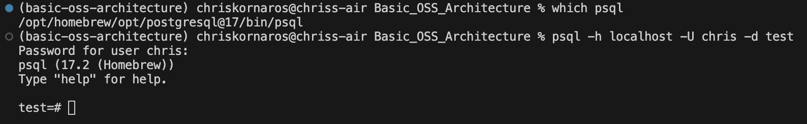
I’m working on a MacOS laptop and manage local packages (like Python, Docker, gh, and Postgres) with Homebrew. Even though I had PostgreSQLv17 installed, it wasn’t added to my PATH for some reason. So, when I ran psql ... I got an error. To fix this, I simply edited the ~/.zshrc (the MacOS default terminal zsh configuration file in my home directory) and added export PATH="/opt/homebrew/opt/postgresql@17/bin:$PATH".
Exploring the Environment
Now that you’re all setup and connected, it’s time to explore the environment and verify your privileges. In this section I’ll run through some basic commands that you can use to understand whatever postgres environment you’re in.
First, the \du command will tell you which roles are available and their attributes:
test=# \du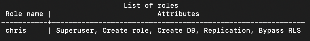
Second, the \l command lists all databases:
test=# \l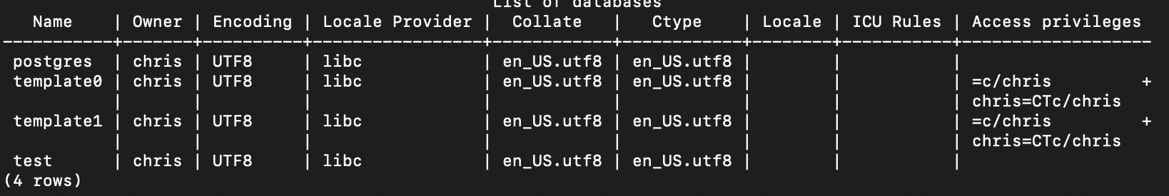
Third, the \dn command lists all schemas:
test=# \dn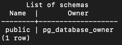
Fourth, the \dt command lists all tables. You should expect this output upon creation of a new database:
test=# \dt
Did not find any relations.
Here are some other useful commands that will not be useful with a fresh database:
\dvlists all views\d table_namelists all columns in a table with name table_name\di table_namelists all indexes for a table with name table_name
Finally, to really dive into a specific database, you’ll use the \c command, but in my case I connected when I first ran the psql command. If you just type psql without the -d flag, you’ll simply connect to a server in general, not a specific database.
At this point, the initial project configuration is just about done. The next steps involve initializing the persistent DuckDB database to use as the Dev/Test environment and defining the raw data model with dbt. For now, you can close the connection to the Postgres server and shutdown container.
The basic data model and ingestion will all be handled in DuckDB and Python.
DuckDB
DuckDB is:
Simple: Easy to install and deploy, has zero external dependencies, and runs in-process in its host app or as a single binary. Portable: Runs on Linux, macOS, Windows, and all popular hardware architectures, has client APIs for major programming languages Feature-rich: Offers a rich SQL dialect. Can read/write files (CSV, Parquet, and JSON), to and from the local file system, and remote endpoints such as S3 buckets. Fast: Runs analytical queries at blazing speed due to its columnar engine, which supports parallel execution and can process larger-than-memory workloads. Extensible: DuckDB is extensible by third-party features such as new data types, functions, file formats and new SQL syntax. Free: DuckDB and its core extensions are open-source under the permissive MIT License.
TL;DR DuckDB is awesome.
As the block of text tells you, while DuckDB is both simple and portable, it is also feature-rich, which is why it’s great for a development or test environment. It’s even easy to spin-up an instance of DuckDB in-memory, while you’re testing or exploring data, and then you can choose to remove that or persist the file in storage.
DuckDB can operate in both persistent mode, where the data is saved to disk, and in in-memory mode, where the entire data set is stored in the main memory. To create or open a persistent database, set the path of the database file, e.g., database.duckdb, when creating the connection. This path can point to an existing database or to a file that does not yet exist and DuckDB will open or create a database at that location as needed. The file may have an arbitrary extension, but .db or .duckdb are two common choices with .ddb also used sometimes. Starting with v0.10, DuckDB’s storage format is backwards-compatible, i.e., DuckDB is able to read database files produced by an older versions of DuckDB. DuckDB can operate in in-memory mode. In most clients, this can be activated by passing the special value :memory: as the database file or omitting the database file argument. In in-memory mode, no data is persisted to disk, therefore, all data is lost when the process finishes.
For more information, here are links to some important pieces of DuckDB:
As you’ll see, I’m planning to use DuckDB with Python to ingest raw data from an API (or flat files) and then build the dbt models based off that (with some help from built-in DuckDB functionality). After that, I’ll connect dbt to Postgres and copy the data model over.
A Persistent Database with DuckDB
As you saw above, it’s very easy to get started with DuckDB. To keep with the structure of the project, I’m going to put the .duckdb file in the root project directory because the Dockerfile (which serves as the Postgres file) is there as well. By design, it’s easy to create a persistent database and manage the file (there’s only one). You have two options:
- Launch DuckDB and create your database file on launch (example below)
- Launch DuckDB, then run
.open test.duckdb
For the purposes of this workflow, it’s better to create the file when you initially launch DuckDB; however, if you are using DuckDB in-memory for EDA or an adhoc ask, but want to persist your work the second option is valid.
Basic_OSS_Architecture % duckdb test.duckdb
v1.1.3 19864453f7
Enter ".help" for usage hints.
D SELECT * FROM duckdb_tables();
.exit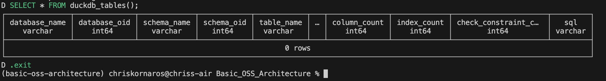
You can then run ls -lh to verify the file exists, and to see some basic file metadata: read/write/executable permissions, author, file size, last edited. Next, I need to configure DuckDB to work with dbt.
dbt
Up to this point, I’ve initialized the project environment and outside of a few lines of code, most of the work has been automated:
- Initialized the project environment with
uvand addedPythonpackages - Initialized the project repository with
gitandGitHub - Initialized the documentation envrionment with
Quarto - Initialized the data model with
dbt - Wrote a
Dockerimage to contain thePostgreSQLserver - Created the test database with
DuckDB
Now, it’s time to start connecting everything, which is exactly what dbt does best.
dbt Core (data build tool) is an open-source framework designed for transforming raw data in a warehouse into a well-structured and actionable format. It operates by enabling analysts and engineers to write modular SQL queries and manage their transformations as code, following software engineering best practices like version control and testing. dbt is used to define, test, and document data pipelines, helping teams standardize and automate transformations in a consistent and scalable way. Key benefits include increased collaboration, improved data quality through built-in testing, and the ability to easily track and manage changes in data models over time. It integrates seamlessly with modern cloud data warehouses, making it a cornerstone for modern data engineering workflows.
Learn more about getting started with dbt.
Configuring Database Connections with dbt
There are two contexts when working with dbt locally: the project dbt directory and the global dbt configuration. The first is what I initialized for the sake of this project using dbt init. The second is the profiles.yml file in the ~/.dbt directory, which is used by dbt to connect to different databases. You’ll also need to install the specific connection type extensions, in this case dbt-duckdb and dbt-postgres– both of these are added like any other dependency with uv add.
The file and folder should be created when you first install dbt-core. If the file isn’t there, you can simply create one. The general syntax is as follows:
basic_oss:
  target: test # The default output for dbt to target (either test or prod in this case)
  outputs: # The defined outputs for dbt to target
    test: # Name of the output
      type: duckdb # Database type
      path: /Users/chriskornaros/Documents/Basic_OSS_Architecture/test.duckdb # Database file path
      schema: ingest # Schema to target
      threads: 4 # The number of threads dbt is allowed to enable for concurrent use
    prod:
      type: postgres
      host: localhost # Hostname of the PostgreSQL server/container
      port: 5432 # Port postgres listens on
      user: chris # User must be specified
      password: # Unfortunately I had to type this in, I haven't found a way to link the key file to profiles.yml yet
      database: test # Database must be specified
      schema: stage # Schema to target
threads: 4 # Threads for concurrencyThreads in a CPU are the smallest units of execution that can run independently, allowing a processor to handle multiple tasks concurrently. They improve performance by utilizing CPU cores more efficiently, especially in multithreaded applications. With Python 3.13, the GIL (global interpreter lock) is gone, you can now actually utilize multiple cores at once. If you want to find out how many cores you have, run sysctl -n hw.logicalcpu (MacOS) or lscpu (Linux).
Logical CPUs represents the number of threads that the system can handle concurrently, a more accurate measure of how many threads your system can execute simultaneously than Physical CPUs because of hyperthreading.
You’ll also need to configure the project specific YAML file– dbt_project.yml. This is easy and, for the most part, the default version of the file that is generated by dbt init is good enough for an initial connection. Later on, I’ll go into some other features and properties that you can define which make dbt even more powerful.
# Name your project! Project names should contain only lowercase characters
# and underscores. A good package name should reflect your organization's
# name or the intended use of these models
name: 'basic_oss'
version: '1.0.0'

# This setting configures which "profile" dbt uses for this project.
profile: 'basic_oss'

# These configurations specify where dbt should look for different types of files.
# The `model-paths` config, for example, states that models in this project can be
# found in the "models/" directory. You probably won't need to change these!
model-paths: ["models"]
analysis-paths: ["analyses"]
test-paths: ["tests"]
seed-paths: ["seeds"]
macro-paths: ["macros"]
snapshot-paths: ["snapshots"]

clean-targets:         # directories to be removed by `dbt clean`
  - "target"
  - "dbt_packages"
  - "logs"

models:
  basic_oss:
    ingest:
      +schema: ingest
      +materialized: table
      +enabled: true
    stage:
      +schema: stage
      +materialized: table
      +enabled: true
Once you have those files configured and saved, you can verify that things were done correctly by running the code below and seeing a similar output to the subsequent image.
Note: It is important that you use uv tool run to execute the command because the dbt-duckdb extension is installed within uv’s project context, not system wide. So, the debug will fail if you just use dbt debug. Additionally, when running from the main project directory, you need to specify the dbt project directory. Otherwise, dbt cannot find the dbt_project.yml file, there is a siimilar flag for the profiles.yml file, if yours is not in your ~/.dbt folder.
Furthermore, while VS Code automatically picks up on uv and its environment, you will need to manually activate the virtual environment if working in a standalone terminal. Even inside of that virtual environment, you will need to use uv tool run
uv tool run dbt debug --profile basic_oss --target test --project-dir basic_oss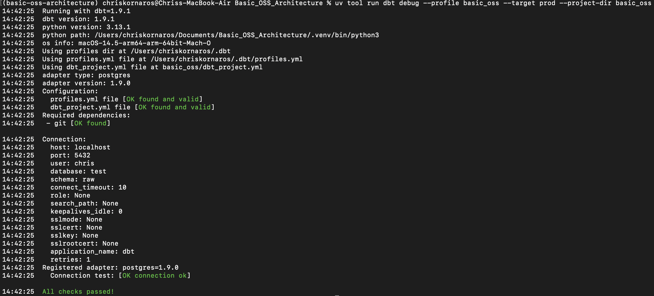
uv tool run dbt debug --profile basic_oss --target prod --project-dir basic_oss 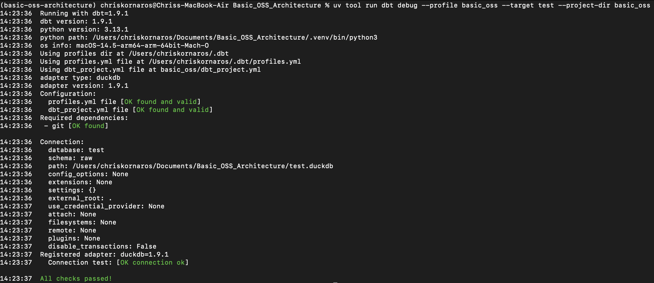
Data Selection and Ingestion
Now that I have the environment good to go, the databases configured, and dbt connected, it’s time to pick a dataset and start building the data model. To do this, I’m first going to add a directory for notebooks (eventually I’ll add one for scripts) and then create a Jupyter notebook. I prefer developing in notebook simply because I can quickly change and test code as I’m iterating. Then, as a reminder, if you haven’t installed the Python dependencies, you can do so with uv add.
In the following block, you’ll see me use code. This command is the VS Code CLI tool, you can learn more here.
mkdir notebooks
code notebooks/api_axploration.ipynb

uv add dbt-core # The core dbt package, needed for base functionality
uv add dbt-duckdb # The DuckDB extension, needed to connect with dbt
uv add dbt-postgres # The postgres extension, needed to conenct with dbt
uv add duckdb # DuckDB Python package
uv add fsspec # Dependency for DuckDB JSON functionality
uv add great-expectations # GX is for data validation/quality, later on
uv add jupyter # Jupyter will launch a Python kernel and makes the notebooks possible
uv add pandas # For standard functionality
uv add pytest # For testing actualy pipeline/script performance, not so much data quality
uv add quarto # For documentation
uv add requests # For making API calls
uv add ruff # An extremly fast Python linter made by Astral, the makers of uv
Configuring and Running a Jupyter Server
Before you can use the notebook, you’ll need to launch and connect to a jupyter server. When developing locally, and not sharing your code or compiled code anywhere, it’s much easier to not require an authentication token. To allow this behavior, you’ll need to modify your jupyter configuration.
I modified my global configuration, because I would have to reconfigure jupyter with every project if I did it in the specific project directory. That being said, I’ll include the local example as well.
# For the global configuration
code ~/.jupyter/jupyter_server_config.py

c.ServerApp.token = '' # Find this in the .py file, set the value to '' which means nothing
# For the local configuration
mkdir .jupyter
code .jupyter/jupyter_server_config.py
c.IdentityProvider.token = ''As you can see, the process is similar, you’ll just manually create the .jupyter/ folder in your project directory first. THe next step is to start the server. Then, you’ll see an ouput similar to the image below. It will tell you useful information like the server address (localhost in this case), version, et cetera; however, you can now leave that terminal window be, it will continue to run in the background. If you need to stop the server, just go back to the window and hit Ctrl-C.
uv run jupyter server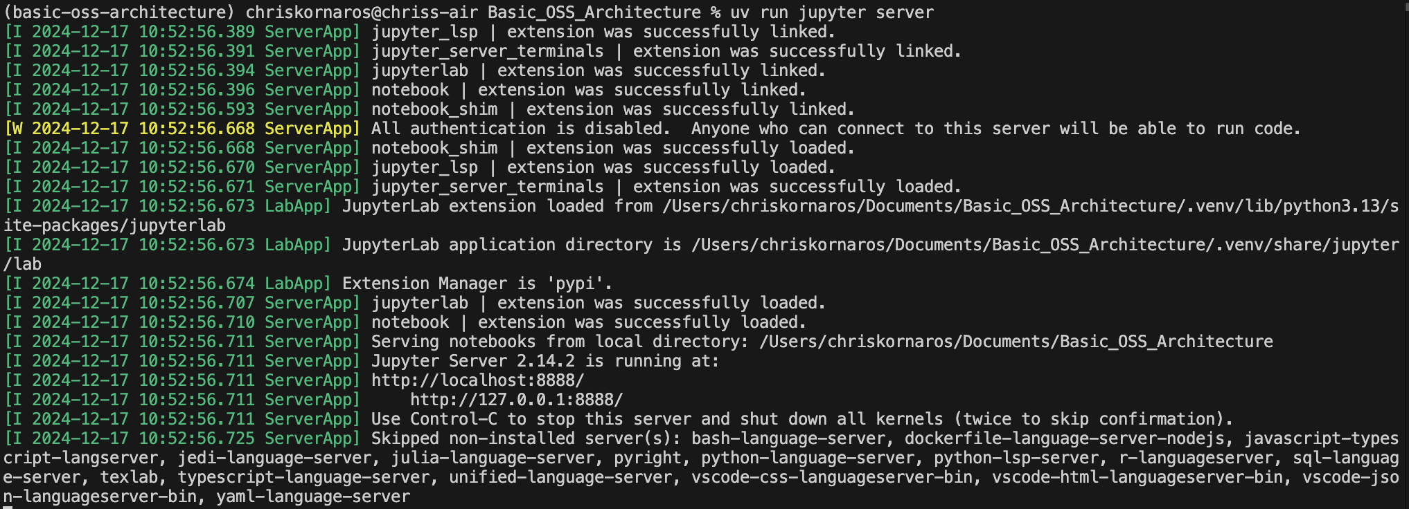
Using The Notebook
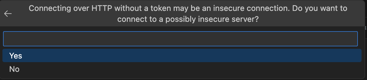
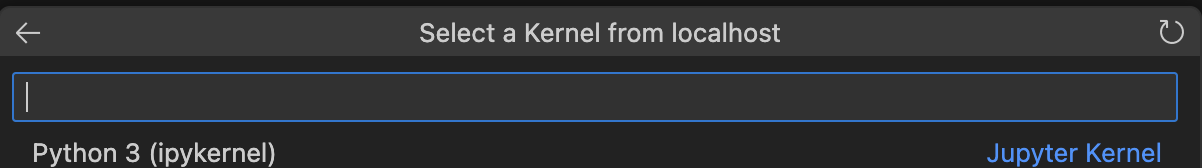
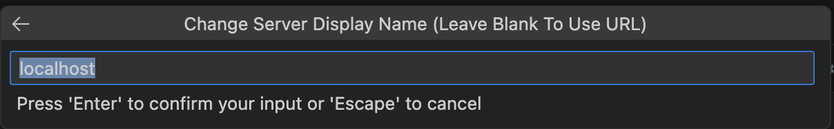
Now that the server is up and running, you can go back to the notebook you created. To use it, I’ll first need to connect to the server (if you see the term kernel don’t be surprised, that’s what a single notebook runs on). Luckily, VS Code provides a really nice UI for connecting a notebook to the Jupyter server. In the images below, I’ll walk you through the connection process. First begin by selecting Select Kernel in the top-right corner of the notebook UI. From there, VS Code’s command palette (the search bar at the top of the window) will interactively walk you through the next steps.
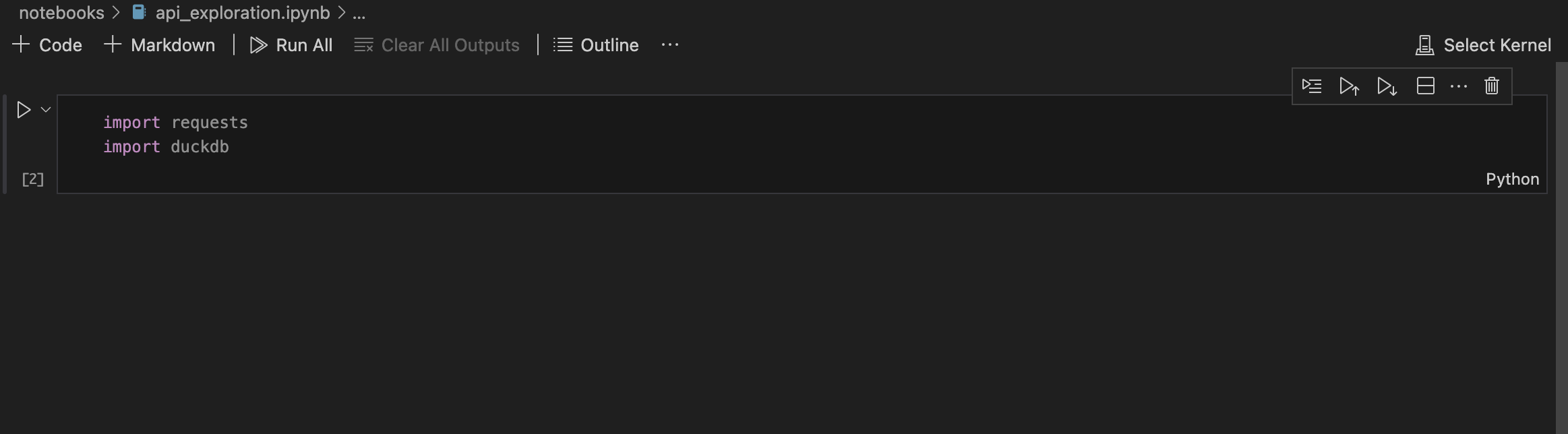

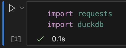
Then, you can verify your connection by running the first cell (Ctrl-Enter on MacOS).
GET-ting my Initial Data
Now that everything is setup and I can actually run Python code within the notebook, it’s time to pick an API and make a request to actually get the data. If you aren’t sure where to start looking for an API, PublicAPI has a great site of publicly available datasets. Many of which are accesible both programmatically or through GUIs.
Before I jump into the code, two quick notes about HTTP and GET:
These are protocols used for transferring data over the internet.
HTTP(HyperText Transfer Protocol) andHTTPS(Secure HyperText Transfer Protocol) are foundational protocols that allow web browsers and servers to communicate with each other. HTTPS adds a layer of security by encrypting the data exchanged between the client and the server.GETis one of the most common HTTP methods used to request data from a specified resource. It retrieves information from the server without making any changes. This method is used when you want to fetch data, such as retrieving data from an API endpoint. It is simple and effective for read-only operations, such as querying data from a database or fetching information from a web service.
Next, you’ll choose the API you want to server as your data source. I decided to use NASA’s NEO (Near Earth Object) Feed for the following reasons:
Dataset:Information about NEOs, including size, orbital path, and speed.API Endpoint:https://api.nasa.gov/neo/rest/v1/neo/browse?api_key={API key}Data Characteristics:JSON structure with a list of NEOs, each containing details like id, name, nasa_jpl_url, absolute_magnitude_h, estimated_diameter, close_approach_date, and more.Use Case:Ideal for a beginner, as it provides a simple JSON structure with basic information and is updated regularly.
Besides my interest in space, the other perk of using NASA’s API is that it’s free and provides a reasonable amount (1,000) of hourly calls. That being said, the documentation isn’t perfect, but it’s definitely easy enough to query. Below, I’ll share the first few cells of my notebook. Learn more on the NASA API Website.
# Import the required packages
import requests
import pprint # pprint similar to beautiful soup, but better for my specific use case
import duckdb
import pandas as pdIf you’re using VS Code, Jupyter notebook context is the parent directory that you opened the file from. In my case code notebooks/api_exploration.ipynb resulted in the context being the root dir above notebooks (Basic_OSS_Architecture/), instead of notebooks. So, I was initially connecting to a persistent DuckDB file created in my Documents directory, instead of the file within my project directory because my connection string below was ../test.duckdb instead of test.duckdb. As a result, I wasn’t able to interact with the environment from my CLI.
# Open a connection to the persistent database
con = duckdb.connect('test.duckdb')
duckdb.install_extension("httpfs") # Lets you directly query HTTP endpoints
duckdb.load_extension("httpfs") # Trying this functionality out to simplify the ETL process

con.sql("SELECT * FROM duckdb_tables()") # Note: Don't use a semi colon in DuckDB for PythonI tried using the httpfs extension from DuckDB to handle the API calls; however, you need a specific file at the location, such as .csv or .parquet. It didn’t work for me, so I ended up doing things differently.
# Store the base API information, for this, I'm using NASA's Near Earth Object (NEO) API
api_key_path = "/Users/chriskornaros/Documents/local-scripts/.api_keys/nasa/key.txt"
with open(api_key_path, 'r') as file:
    api_key = file.read().strip()
start_date, end_date = "2024-12-01", "2024-12-04"

# Then Construct the URL with f-string formatting
url = f"https://api.nasa.gov/neo/rest/v1/feed?start_date={start_date}&end_date={end_date}&api_key={api_key}"
# Standalone cell for the API response, ensures I don't call too many times
response = requests.get(url)
# Check if the response was successful, if so, print the data in a human readable format
if response.status_code == 200:
data = response.json()
pprint.pprint(data)
else:
print(f"Error: {response.status_code}")Creating the Raw Table
Now that you’ve successfully connected to the API and made your first GET request, it’s time to get the API output in a format that DuckDB can read into a table. If your API output is anything like mine, it’ll be messy, even with the help of pprint, as you can see below. So, before I can create the table, I need to flatten the dictionary output.
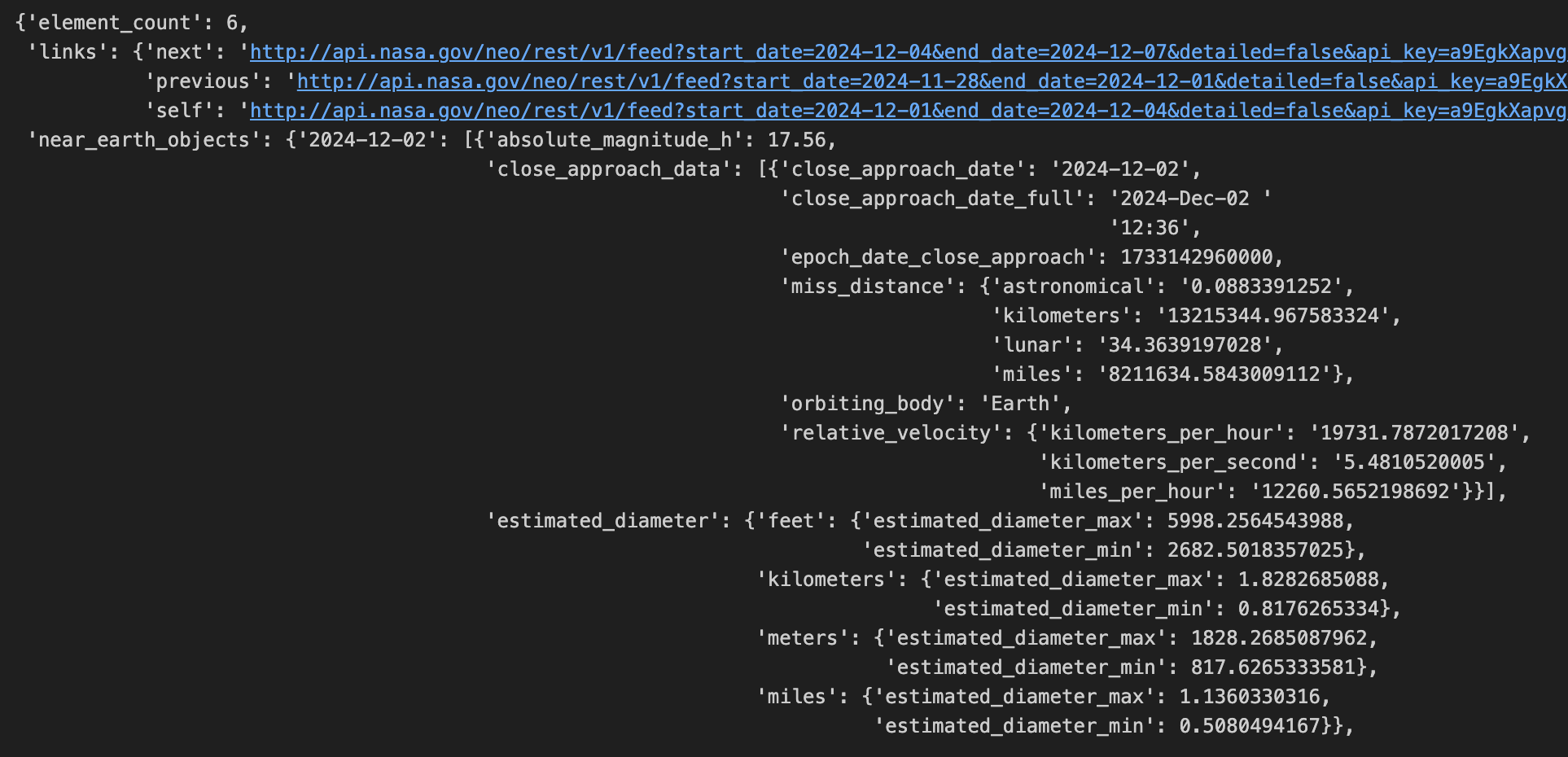
Luckily, there are some simple functions in both Python and DuckDB that can help.
# Flatten the output and then read it with DuckDB to get the column data types
flat_data = pd.json_normalize(data['near_earth_objects']['2024-12-02'])

raw = con.sql("""CREATE TABLE asteroids AS
                SELECT * EXCLUDE(nasa_jpl_url, close_approach_data, 'links.self')
                , unnest(close_approach_data, recursive := true)
                FROM flat_data
                """)

con.sql("SELECT * FROM duckdb_tables()") # Shows table metadata, validates the script worked as intended
What flat_data did is tell Python that the dictionary values for the key ‘near_earth_objects’ are what I’m looking for and to get rid of the rest of the information, while elevating the nested hierarchy. It takes that one step further, by specifying the actual date (which are the keys in this dataset). That results in an output that you can view below; however, there is still a column with the DuckDB [struct](https://duckdb.org/docs/sql/data_types/struct) type. Simply put, the struct type is similar to tuples in Python because the data type is actually an ordered list of columns called entries. These entries can even be other lists or structs.

So, I’ll need to further flatten my dataset. Luckily DuckDB SQL provides a native function for this exact behavior, UNNEST, and lets me execute it in the same statement I’m creating a table! This effectively does what flattening with Python functions does, the nice thing is you can set the recursive := parameter to true, letting DuckDB also handle nested structs, within a struct. As you can see, the DuckDB query selects everything except for the data source’s GUI URL, the original struct data, and the API query for the specific NEO object in that row.
Now that the table structure is done and ready for data. It’s time to finish off some final configurations for our dbt project. Both files will go in the models/ folder, namely schema.yml and sources.yml. Here’s a quick note on the purpose of both.
schema.yml
The schema.yml file documents and tests the models and columns created within your dbt project, ensuring data quality and consistency. It allows you to define metadata, such as column descriptions, and add constraints like uniqueness or nullability tests to enforce integrity. This fosters trust in your data pipelines, simplifies debugging, and enhances the readability of your data models for developers and stakeholders.
version: 1

models:
  - name: asteroids
    description: "A table containing detailed information about near-Earth objects, including their estimated dimensions and close approach data, in metric units."
    columns:
      - name: id
        description: "Unique identifier for the asteroid."
      - name: neo_reference_id
        description: "Reference ID assigned by NASA's Near Earth Object program."
      - name: name
        description: "Name or designation of the asteroid."
sources.yml
The sources.yml file defines the external data sources your dbt project depends on, such as raw tables or views in your database, and ensures their existence and structure are tested before being used. It helps you document where your data originates, making your project more transparent and easier to maintain. By validating source data and organizing dependencies, it reduces the risk of downstream errors and improves collaboration across teams.
version: 1

sources:
  - name: ingest
    description: "Data in its base relational form, after being unnested from the API call"
    database: basic_oss
    schema: ingest
    tables:
        - name: raw
          description: "A table containing the non-formatted API data"
          columns:
            - name: id
              description: "Unique identifier for the asteroid."
            - name: neo_reference_id
              description: "Reference ID assigned by NASA's Near Earth Object program."
            - name: name
              description: "Name or designation of the asteroid."
Creating dbt models
Now that the dbt project is configured and I did some feature testing in a notebook, it’s time to actually write the models which will serve as the tables in our database. The sources and schema files live in the models/ directory. Within the models folder, you’ll create subfolders that will house your actual models. I use these subfolders to group models by schema. I’m going to have two schemas with one model each, initially, to showcase some dbt features.
ingest/will house the model that calls the API and creates the table.stage/will house the data transformations necessary to get the table in a useful state
The nice thing about DuckDB is that you can directly query files on the internet. Unfortunately, the NASA API I’m calling returns the data as text, not a file. So, I’ll need to use Python to make the initial call and fetch the raw data. Luckily, as of dbt-core v1.3, you can now add .py files as dbt models. So, the first step, after creating the models subdirectories, is to convert the code in the Jupyter notebook to a Python script.
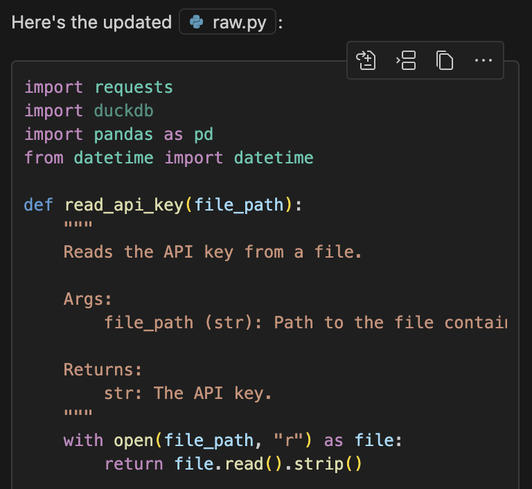
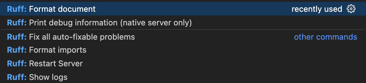
Fortunately, as of writing this, GitHub Copilot is now free. So, I was able to easily convert the file and then check it using ruff in about 10 seconds. Copilot lets you define the context you’re working in, so I had it look at the notebook file and the raw file. Then, after making some slight changes (because of specific dbt functionality) I was able to click a button and have Copilot paste the code in the editor. Finally, I used ruff to check the file for any errors and format it. I’ll share images below.
Python Model
It’s important to know that the actual model has a specific format and output requirement. As you’ll see below, instead of a main function, I created a model(dbt, session) function. It’s similar to a main function, but is specific for enabling dbt to read Python. Furthermore, the entire .py file needs to output one single DataFrame.
# Import the required dependencies
import requests
import duckdb
import pandas as pd
from datetime import datetime, timedelta


def read_api_key(file_path):
    """
    Reads the API key from a file.

    Args:
        file_path (str): Path to the file containing the API key.

    Returns:
        str: The API key.
    """
    with open(file_path, "r") as file:
        return file.read().strip()


def construct_url(api_key, start_date, end_date):
    """
    Constructs the API URL.

    Args:
        api_key (str): The API key.
        start_date (str): The start date for the API query.
        end_date (str): The end date for the API query.

    Returns:
        str: The constructed API URL.
    """
    return f"https://api.nasa.gov/neo/rest/v1/feed?start_date={start_date}&end_date={end_date}&api_key={api_key}"


def fetch_data(url):
    """
    Fetches data from the API.

    Args:
        url (str): The API URL.

    Returns:
        dict: The JSON response from the API.

    Raises:
        Exception: If the API request fails.
    """
    response = requests.get(url)
    if response.status_code == 200:
        return response.json()
    else:
        raise Exception(f"Error: {response.status_code}")


def process_data(data):
    """
    Processes the API response data.

    Args:
        data (dict): The JSON response from the API.

    Returns:
        DataFrame: The processed data as a pandas DataFrame.
    """
    all_data = []
    for date in data["near_earth_objects"]:
        flat_data = pd.json_normalize(data["near_earth_objects"][date])
        all_data.append(flat_data)

    if all_data:
        final_data = pd.concat(all_data, ignore_index=True)
    else:
        final_data = pd.DataFrame()

    return final_data


def store_data_in_duckdb(con, data):
    """
    Stores the processed data in DuckDB.

    Args:
        con (duckdb.DuckDBPyConnection): The DuckDB connection.
        data (DataFrame): The processed data.
    """
    con.sql("""
        CREATE TABLE IF NOT EXISTS asteroids AS
        SELECT * EXCLUDE(nasa_jpl_url, close_approach_data, 'links.self')
        , unnest(close_approach_data, recursive := true)
        FROM data
    """)


def main():
    """
    Main function to execute the data ingestion process.
    Returns a single DataFrame object.
    """
    api_key_path = "/Users/chriskornaros/Documents/local-scripts/.api_keys/nasa/key.txt"
    api_key = read_api_key(api_key_path)

    # Define the start date and end date for the 7-day window
    start_date = datetime.strptime("1900-01-01", "%Y-%m-%d")
    end_date = start_date + timedelta(days=7)

    url = construct_url(
        api_key, start_date.strftime("%Y-%m-%d"), end_date.strftime("%Y-%m-%d")
    )

    try:
        data = fetch_data(url)
        final_data = process_data(data)
    except Exception as e:
        print(f"Failed to fetch data: {e}")
        final_data = pd.DataFrame()

    # Open a connection to the persistent database
    con = duckdb.connect("test.duckdb")

    # Store the data in DuckDB
    store_data_in_duckdb(con, final_data)

    # Verify the data was stored correctly
    result = con.sql("SELECT * FROM asteroids").fetchdf()
    print(result)

    # Close the connection
    con.close()

    return final_data


if __name__ == "__main__":
    df = main()
    print(df)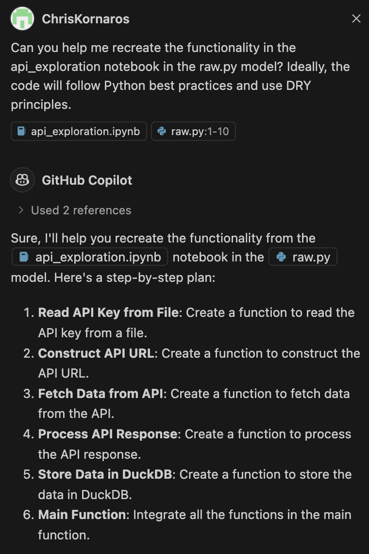
ruff check
# All checks passed!
SQL Model
Next, I’m going to create a simple SQL model to only use the metric data from the table. Additionally, the model cleans up some column names.
-- Column names and data types taken from the API Exploration Notebook
WITH a_raw AS (
    SELECT *
    FROM main.asteroids
)

SELECT id, neo_reference_id, name, close_approach_date, close_approach_date_full, epoch_date_close_approach
    , absolute_magnitude_h, is_potentially_hazardous_asteroid, is_sentry_object
    , kilometers_per_second, kilometers_per_hour, kilometers_miss, orbiting_body
    , "estimated_diameter.kilometers.estimated_diameter_min" AS km_estimated_diameter_min
    , "estimated_diameter.kilometers.estimated_diameter_max"AS km_estimated_diameter_max
    , "estimated_diameter.meters.estimated_diameter_min" AS meters_estimated_diameter_min
    , "estimated_diameter.meters.estimated_diameter_max" AS meters_estimated_diameter_max
FROM a_raw
Running your models
Now that everything is ready, it’s finally time for dbt to shine! To ensure functionality, as I expect it, I like to cd dbt_dir/ before running the models. Then, once I’m in the dbt project directory, all I have to do is execute dbt run from my CLI for DBT to start exectuing scripts. That being said, if you only want to test or run a specific model, you can tell dbt exactly which folder to look at using dbt run --select ingest. Just know, even though you may only run one specific folder, dbt will throw an error if there is an issue with a model in another subfolder.
Next Steps
- Setup my Raspberry Pi server so I have an always-running VM for job orchestration
- Setup Airflow to schedule the jobs, so every 15 minutes the API is called
- This won’t break the API rules and will take about 2 months to get all existing data
- Continue with the rest of the vision/integrations